shady_amsterdam
Pedestrian Network Analysis
Pedestrian Network Analysis part offers a set of tools designed to identify shaded paths, locate shaded (cool) places, and map proximity to cool places around buildings.
Using these tools, users can:
- Calculate shaded routes between two locations or to the nearest cool place, optimizing for either distance or shade.
- Generate a walking shed network that classifies buildings based on their proximity to cool places, providing insights into accessible shaded zones within the city.
Each module functions independently, allowing users to perform dataset preparation, routing, or walking shed analysis based on their needs.
Content
- 1.1. Shade Weight Calculation (shade_weight_calculation.py)
- 1.2. Cool Places Nodes Calculation (cool_places_nodes_calculation.py)
2. Routing (routes_calculation.py)
3. Walking Shed Network (walking_shed_network.py)
1. Dataset Preparation
The dataset preparation phase includes calculating shade weights for pedestrian network edges and identifying nodes that could represent cool places. This provides foundational data for routing and walking shed calculations.
1.1 Shade Weight Calculation (shade_weight_calculation.py)
How Shade is Calculated
- Overlaying Shade Maps:
- Each shade map is a raster image with pixel values indicating shaded and non-shaded areas.
- The script overlays each edge in the network with the raster to determine the amount of shade along that edge.
- Using Zonal Statistics:
- For each edge, zonal statistics are applied to calculate two values:
- Sum of Pixel Values: The total shade in the edge’s area.
- Count of Pixels: The total number of pixels in the edge’s area, representing its overall size.
- For each edge, zonal statistics are applied to calculate two values:
- Calculating Shade Proportion:
- The shade proportion for each edge is calculated as: shade proportion = (count of pixels - sum of pixel values) / count of pixels
- A higher shade proportion means more of the edge is shaded, while a lower proportion indicates less shade.
- Converting Shade Proportion to Shade Weight:
- To prioritize shaded paths, the shade weight is calculated as the inverse of the shade proportion: shade weight = 1 / (shade proportion + 1e-5)
- This formula gives shadier edges a lower shade weight, making them more favorable in shaded route calculations. A small constant (1e-5) is added to avoid division by zero.
- Default Weight:
- If no shading information is available for an edge, a high default weight (e.g., 1000) is assigned, making it less likely to be selected in shaded routing.
Entry Function: process_multiple_shade_maps(graph_file, raster_dir, output_dir)
The entry function process_multiple_shade_maps calculates shade weights for all edges in a network based on raster shade maps.
How to Use:
- Set the
graph_fileto specify the pedestrian network. - Provide
raster_dirwith the shade maps in.TIFformat. The shade maps should have file names asxxx_YYYYMMDD_HH,such asamsterdam_20241031_900. - Specify
output_dirto save the updated GraphML files.
Example:
process_multiple_shade_maps(graph_file="path/to/network.graphml", raster_dir="path/to/shade_maps", output_dir="path/to/output")
Notes: While in json configuration file, for convenience, an area name could also be provided. With an area name, the program will automatically obtain OSM network of a certain area.
1.2 Cool Places Nodes Calculation (cool_places_nodes_calculation.py)
How Cool Place Nodes Are Identified
- Load the Network and Cool Place Polygons:
- The script starts by loading a pedestrian network graph and a set of polygons representing cool places (from a shapefile).
- Polygons are validated and, if necessary, repaired to ensure all geometries are valid.
- Convert Nodes and Polygons for Spatial Analysis:
- The network’s nodes are converted to a GeoDataFrame and projected to a known coordinate system (e.g., EPSG:28992).
- The polygons representing cool places are also re-projected to match the network nodes, enabling accurate distance calculations.
- Efficient Distance Lookup with KDTree:
- A KDTree is created from the node coordinates, allowing fast nearest-neighbor searches.
- For each cool place polygon, key points around the polygon’s boundaries (bounding box corners) are identified for querying nearby nodes.
- Finding Nearby Nodes:
- Using the KDTree, nodes within a maximum distance (e.g., 50 meters) of each polygon are identified.
- These nodes represent areas close to or within the cool place polygons and are added to the list of cool place nodes.
- Save Cool Place Nodes:
- The final list of cool place nodes is deduplicated and saved to a
.pklfile, allowing it to be reused for routing or analysis.
- The final list of cool place nodes is deduplicated and saved to a
This module identifies and saves nodes in the pedestrian network that are closest to the bounding boxes of shaded areas, referred to as “cool places”, for further use in route calculations.
Entry Function: process_all_geopackages_in_directory(gpkg_directory, graph_directory, shapefile_output_directory, output_directory)
How to Use:
- Set
gpkg_directoryto the directory containing the GeoPackage files, each named to include a date, such asshadeGeoms_YYYYMMDD.gpkg. - Set
graph_directoryto the directory where shade-weighted GraphML files are located. - Provide
shapefile_output_directoryto specify where to save individual layers exported from each GeoPackage as shapefiles. - Set
output_directoryto save the resulting files containing nodes identified as cool places.
Example
process_all_geopackages_in_directory(
    gpkg_directory="path/to/geopackage_files",
    graph_directory="path/to/graph_files_with_shade",
    shapefile_output_directory="path/to/exported_shapefiles",
    output_directory="path/to/output_cool_place_nodes"
)
2. Routing (routes_calculation.py)
The routing module provides options for calculating the shortest, shadiest, or balanced routes between two locations or to the nearest cool place. This section supports flexible routing configurations based on parameters set in the configuration.
How Routes Are Calculated
- Load the Network and Cool Place Nodes:
- The script begins by loading a network graph with shade weights from a GraphML file.
- Pre-calculated cool place nodes are loaded, representing cool places on the network.
- Identify Start and End Points:
- For route calculations, users can specify coordinates, location names, or choose the nearest cool place as a destination.
- Using spatial queries, the nearest network nodes to these start and end locations are identified.
- Calculate Different Route Types:
- The script calculates four types of routes:
- Shortest Route: The route with the minimum distance between the start and end nodes.
- Shadiest Route: The route that maximizes shade along the path, using the shade weight of each edge.
- Balanced Route 1 (70% Shade, 30% Distance): A route balancing shade and distance with a 70/30 weighting.
- Balanced Route 2 (30% Shade, 70% Distance): A similar route but with a 30/70 weighting between shade and distance.
- The script calculates four types of routes:
- Balancing Shade and Distance:
- For balanced routes, the edges in the network are normalized by their total length and shade weight.
- A custom weighted sum is then calculated based on defined ratios (e.g., 70/30 for shade/distance), creating a balanced route that takes both factors into account.
- Route Visualization:
- If routes are found, they are visualized on a map, showing different colors for each type of route:
- Shortest Route: Blue
- Shadiest Route: Green
- Balanced Route 1 (70% Shade): Purple
- Balanced Route 2 (30% Shade): Pink
- If routes are found, they are visualized on a map, showing different colors for each type of route:
Entry Function Options
The routing process determines which function to call based on the provided configuration:
demo_shade_route_calculation: Uses specific GraphML and nodes files for direct routing.demo_shade_route_calculation_with_time: Searches directories to find the nearest timestamped files for time-based routing.
How to Use:
- Configure either
graph_fileandnodes_filefor direct routing, orgraph_dirandnodes_dirto use directory search for timestamped files. - Set
route_optionto define the routing mode:"nearest_cool_place": Calculates the path to the nearest cool place."origin_destination": Routes between two specified points.
- Set
location_indication_optionto define the location input type:"location_name": Uses location names fororigin_nameanddestination_name."coordinates": Uses coordinates (origin_latitude,origin_longitude, etc.).
- Optionally, specify
date_timeif using directory-based search withdemo_shade_route_calculation_with_time.
Example
Example using specified files for direct routing:
routing_config = {
    "graph_file": "path/to/specific_graph.graphml",
    "nodes_file": "path/to/specific_nodes.pkl",
    "route_option": "origin_destination",
    "location_indication_option": "location_name",
    "origin_name": "Amsterdam Central Station",
    "destination_name": "Dam Square",
}
Output Example
One possible routing output example:
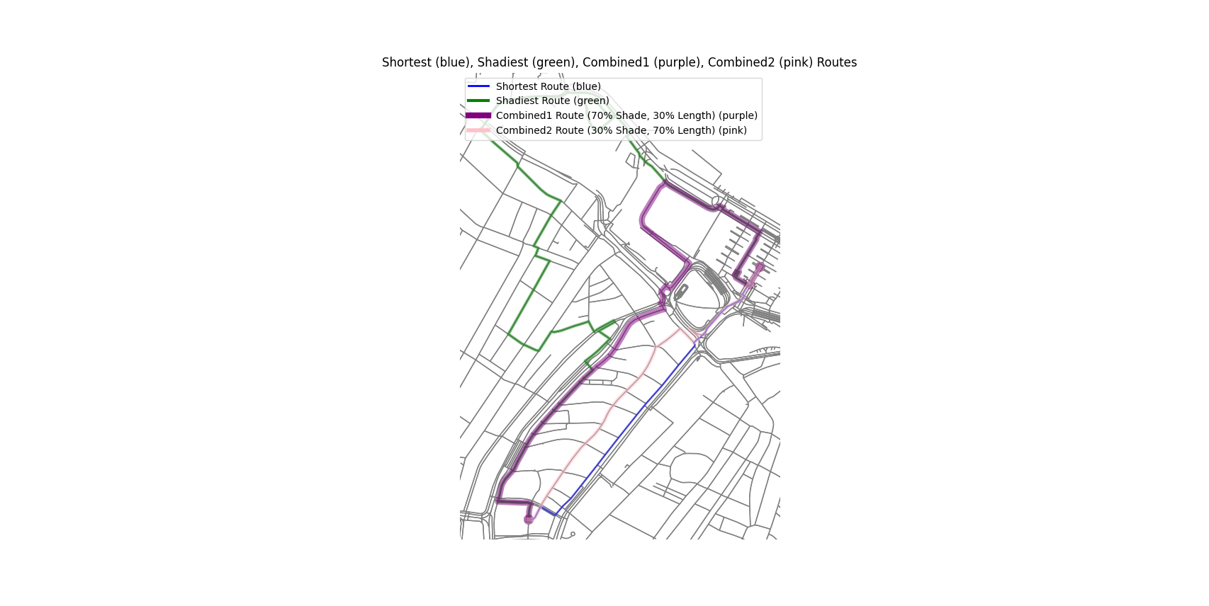
Figure 1: Routing between two locations: Amsterdam Central Station, Dam Square
3. Walking Shed Network (walking_shed_network.py)
The walking shed network analysis categorizes buildings based on their shortest/shadiest distance from cool places, creating a “walking shed” that highlights proximity to cool places.
How the Walking Shed Network is Calculated
- Load the Network, Buildings, and Cool Place Polygons:
- The script loads a pedestrian network graph, a set of polygons representing cool places, and building polygons.
- Each dataset is projected to a consistent coordinate system to ensure accurate distance calculations.
- Identify Cool Place Nodes:
- For each cool place polygon, nearby nodes on the network are identified based on a maximum distance threshold (e.g., 50 meters). These nodes represent access points to cool places.
- Classify Nodes by Distance:
- Using parallelized Dijkstra’s algorithm, the script calculates distances from each cool place node across the network.
- Nodes are classified into distance categories (e.g., 200m, 300m, 400m, 500m) based on their shortest/shadiest distance from a cool place node.
- Assign Distance Categories to Buildings:
- For each building, the nearest network node is identified, and the building is assigned a distance category based on the closest cool place node.
- Buildings farther than the specified maximum distance (e.g., 500m) are placed in an “>500m” category.
- Assign Colors to Distance Categories:
- Buildings are assigned colors based on their distance to the nearest cool place:
- Green: < 200m
- Blue: 200m - 300m
- Yellow: 300m - 400m
- Orange: 400m - 500m
- Red: > 500m
- Buildings are assigned colors based on their distance to the nearest cool place:
- Visualize the Walking Shed:
- The walking shed is visualized on a map, displaying each building in its assigned color.
- Save Output Shapefiles:
- Optionally, the processed buildings and cool place nodes can be saved as shapefiles, enabling further analysis or visualization in GIS software.
Entry Function: walking_shed_calculation(graph, polygon_path, building_shapefile_path, weight="shade_weight", output_building_shapefile=None, output_cool_place_shapefile=None)
How to Use:
- Set
graphto the path of the GraphML file that has been preprocessed with shade weights. - Specify
polygon_pathwith the shaded area polygons in shapefile format. - Provide
building_shapefile_pathfor the buildings layer to categorize buildings by proximity to cool places. - Optionally, specify paths for
output_building_shapefileandoutput_cool_place_shapefileto save results.
Example
walking_shed_calculation(
    graph="path/to/network_with_shade.graphml",
    polygon_path="path/to/cool_places.shp",
    building_shapefile_path="path/to/buildings.shp",
    weight="shade_weight",
    output_building_shapefile="path/to/output_buildings.shp",
    output_cool_place_shapefile="path/to/output_cool_places.shp"
)
Output Example
One possible walking shed output example with shade_weight as weight:
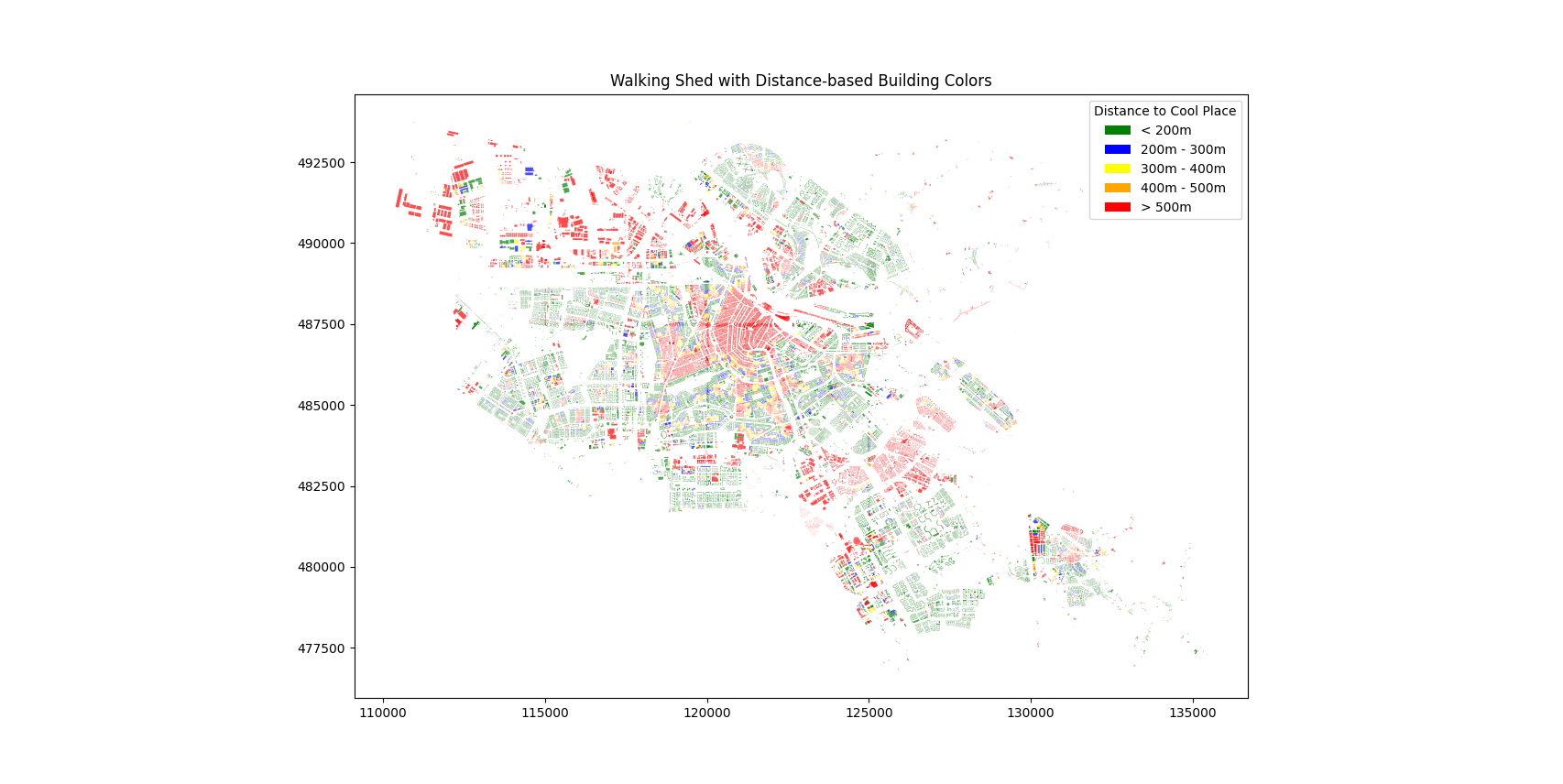
Figure 2: Walking shed with `shade_weight` as `weight`