shady_amsterdam

Cool Space Process

This documentation will explain each step involved in the cool space process, separated in two parts: identification and evaluation. All steps can be performed automatically by running ./cool_place/main.py or main.py with a configuration file containing the required parameters. Information about this configuration file can be found at setting up the Configuration File

All data used for the cool space process must be specified by the configuration file, and all vector data should be Geopackage files (gpkg).

---

Content

1. Data preparation

• 1.1. Land use data
• 1.2. Road data
• 1.3. Building and residential data
• 1.4. Street furniture data
• 1.5. Heat risk data
• 1.6. PET data
• 1.7. shade maps data

2. Identification

3. Evaluation

---

1. Data preparation

For performing cool space process, there are eight datasets used as inputs. Six of them are vector data, stored within one Geopackage as different layers, the two of them are raster datasets.

1.1 Land use data

The land use data are polygons with an attribute to specify different land use type, as shown in figure 1 below.

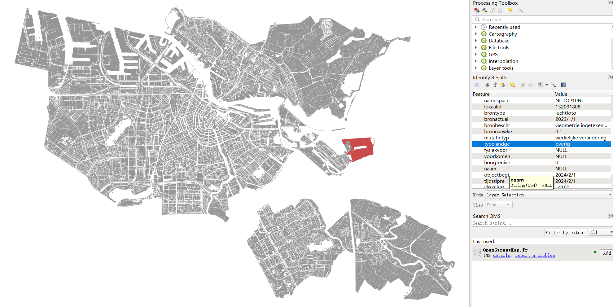
Figure 1: Land use data

1.2 Road data

The road data are polygons with an attribute specifing the buffer number of each polygon, as shown in figure 2 below. The buffer attribute must be numeric attribute.

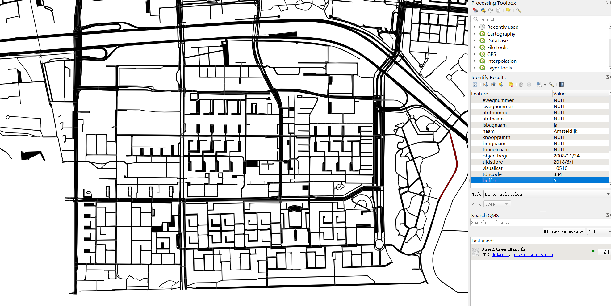
Figure 2: Road data

Note: the program provided includes code to create this buffer attribute, which can only be used for the specific road dataset we provide. For more general road data, there is one line of the code that needs to be muted in the coolspace_process.py:

Figure 3: Code needs to be muted for more general road datasets

1.3 Building and residential data

For building and residential data (building population data), they can be one dataset, which are building polygons containing an attribute of the number of residents within each building, shown in figure 4 below. Note: the attribute name must be resident

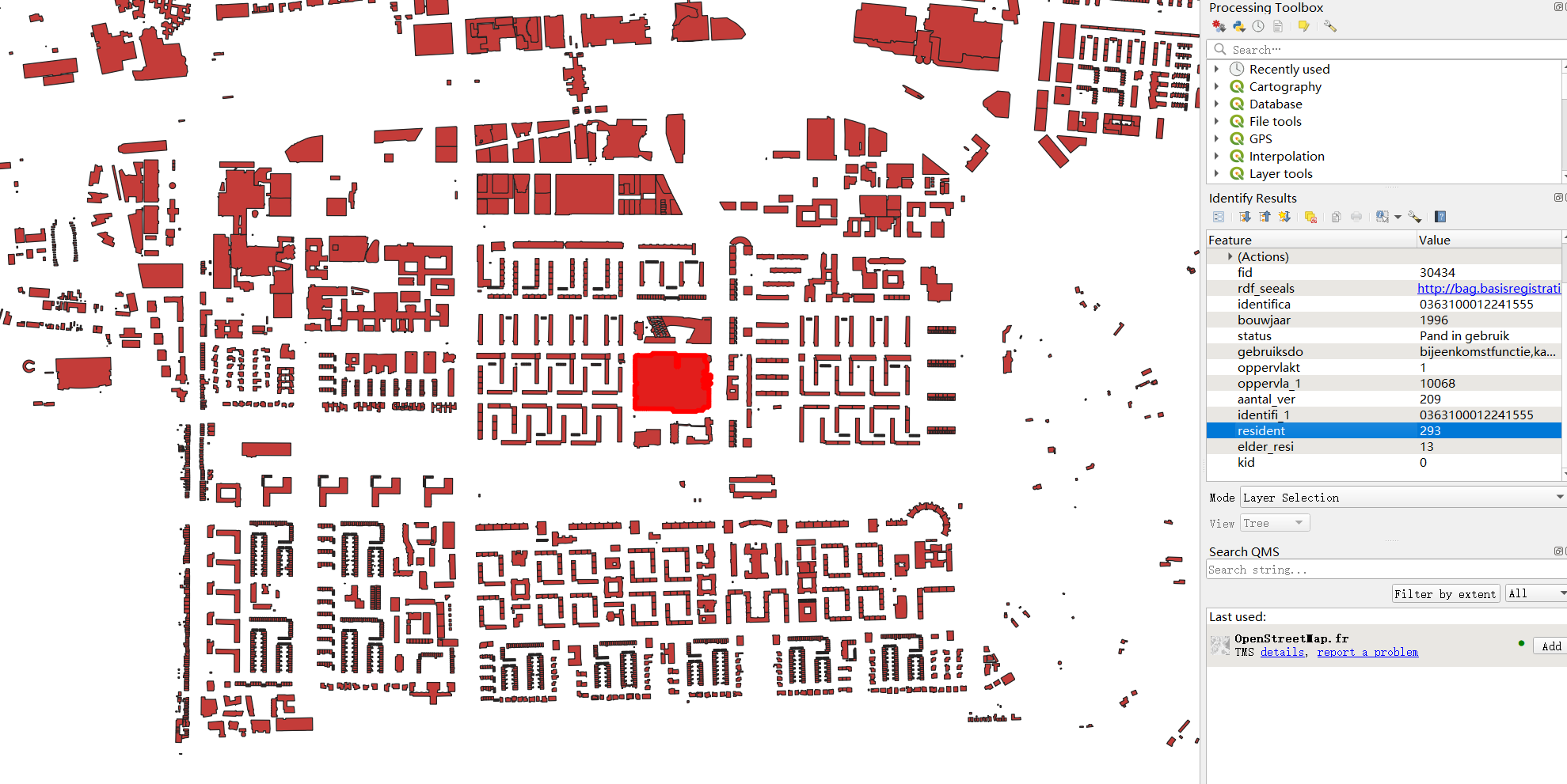
Figure 4: Building data with residents attribute

In the given coolspaceConfig.json, the building data and building population data are two different files, but they can be the same data. Thus simply assign the same file name to building_file and building_population_file parameters in the config file if they are the same.

1.4 Street furniture data

The street furniture data used in this project is the bench data downloaded from OpenStreetMap, which is a point dataset as shown in figure 5. Each point represents the location of a public bench. For the process, no attribute is needed, only the points.

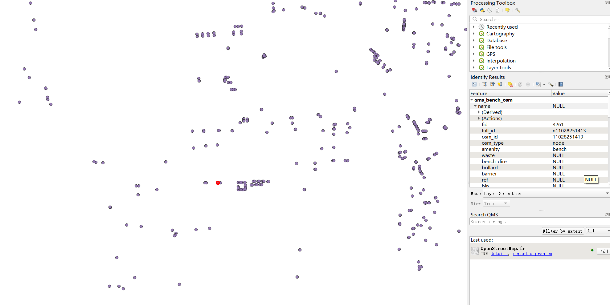
Figure 5: Bench points data

1.5 Heat risk data

The heat risk data are polygons of neighborhood level, containing an attribute named HI_TOTAAL_S which specifys the heat risk level of each neighborhood polygon, as shown in figure 6. Note that the program doesn’t have an input parameter allowing user to set the heat risk attribute name, which means for other heat risk datas, they also have to use the same attribute name HI_TOTAAL_S.

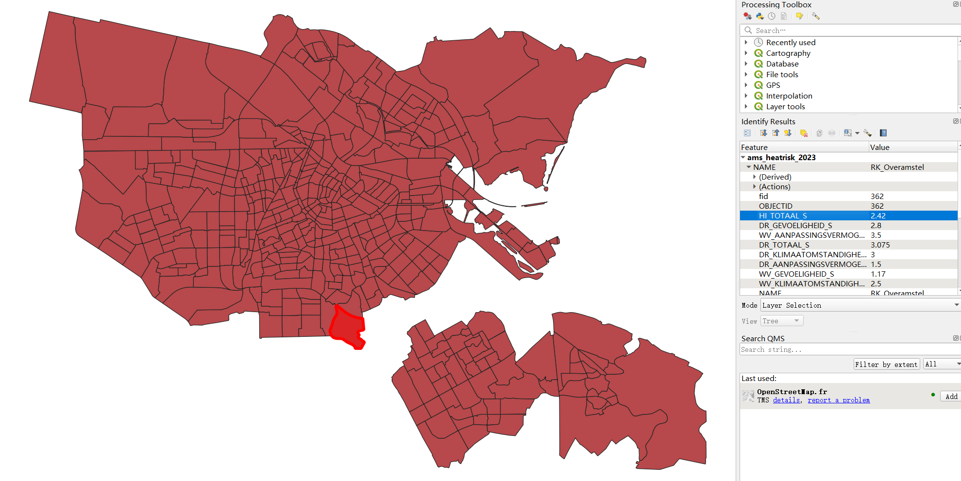
Figure 6: Heat risk data

1.6 PET data

The PET data is a raster data with one band as shown in figure 7, which is a continuous field specifying the Physiological Equivalent Temperature.

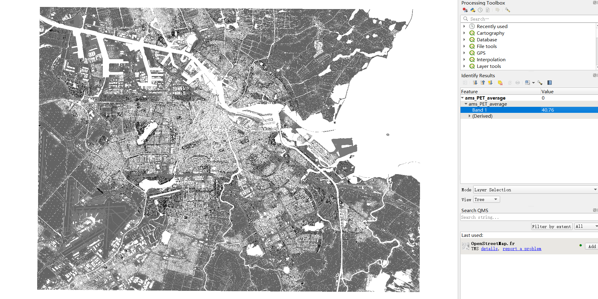
Figure 7: Heat risk data

1.7 Shade maps data

The shade maps are the output from the Shade calculation step, which is a folder contatining all shade maps of the day, from 9:00 to 20:00 as shown in figure 8. The user needs to specify the folder path in the coolspaceConfig.json, telling the program to read shade maps from that folder.

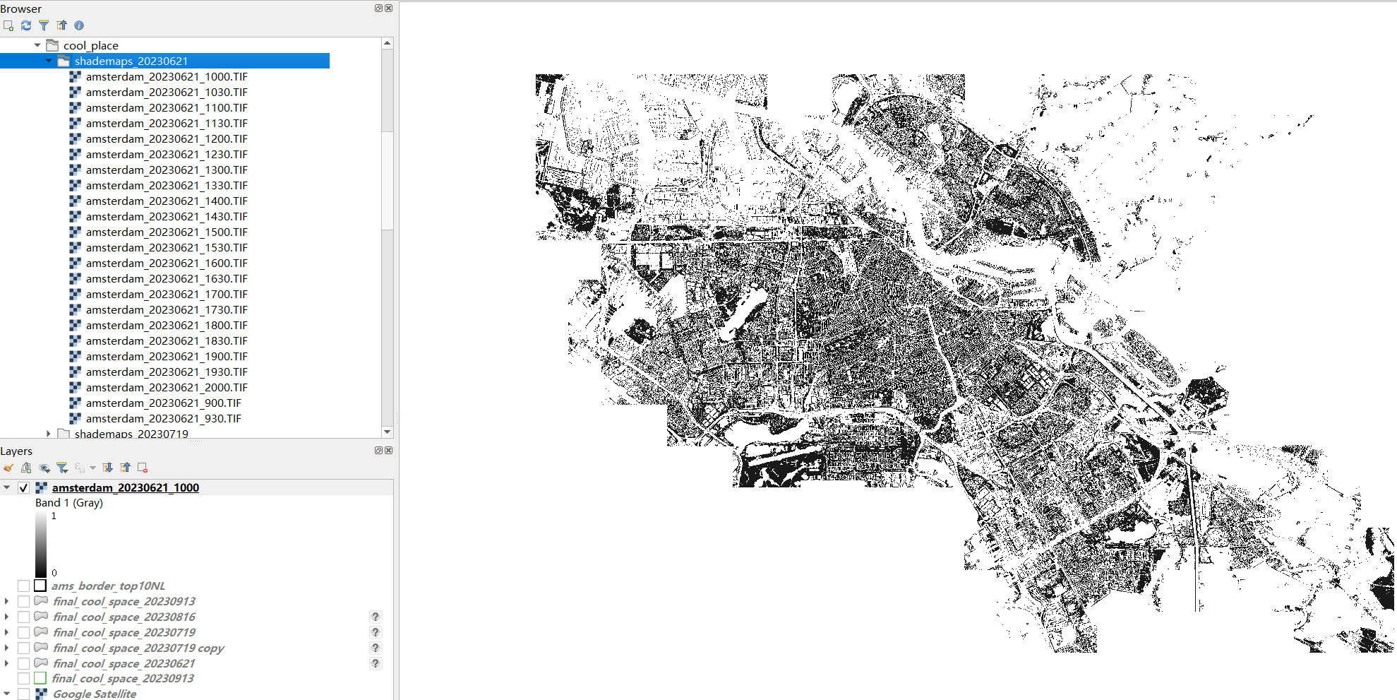
Figure 8: Shade maps

Note that in the screenshot, the file order is not from 900 to 2000, therefore in coolspace_process.py, there is one line of code to sort the input files based on the file name: line 87: shadow_files.sort(key=lambda x: int(os.path.splitext(os.path.basename(x))[0].split('_')[-1])), which means the suffix of shade map name has to be _XXX, where XXX represents the time. Then, the reading order of shade maps is correct which means the program will read from 900 to 2000, having a correct list order, take the screenshot as an example:

• shademaps[0] will be amsterdam_20230621_900
• shademaps[1] will be amsterdam_20230621_930
• shademaps[2] will be amsterdam_20230621_1000
• …

2. Identification

For identification, the program runs as:

• Read road data, building data, land use data and shade maps in main.py of cool space
• Call the identification function in coolspace_process.py
• The public space polygons will be created as a GeoDataFrame from road data, building data and land use data.
• For each shade map, corresponding shaded area within public spaces will be extracted and evaluated, resulting in several new attributes stored back into the public space geodataframe, which are:
  • sdAvg{index}: the average shade value of all shaded areas within a public space
  • sdArea{index}: a list contains the areas of every shaded area within a public space
  • sdGeom{index}: the geometry of shaded areas within a public space, either a polygon or a multi-polygon
• After all shade maps have been processed, the shade coverage indicator will be evaluated, resulting in:
  • scDay and spDay: daytime range shade coverage score
  • scMorn and spMorn: morning time range shade coverage score
  • scAftrn and spAftrn: afternoon time range shade coverage score
  • scLtAftrn and spLtAftrn late afternoon time range shade coverage score
  • sc is the score in terms of time, and sp is the score in terms of area ratio
• Finally, the public space data will be output to the INPUT Geopackage as a new layer, which then be used as input of evaluation part. By default, the public space polygons will be set as active geometry, as shown in figure 9. The user can change the geometry type to land use, which will result in output shown in figure 10.

---

OUTPUT

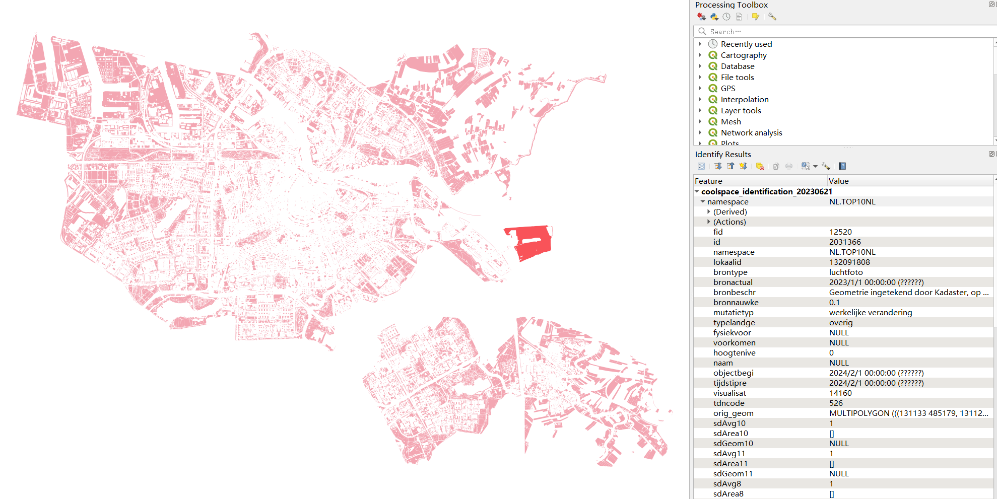
Figure 9: Identification output, geometry type: public space

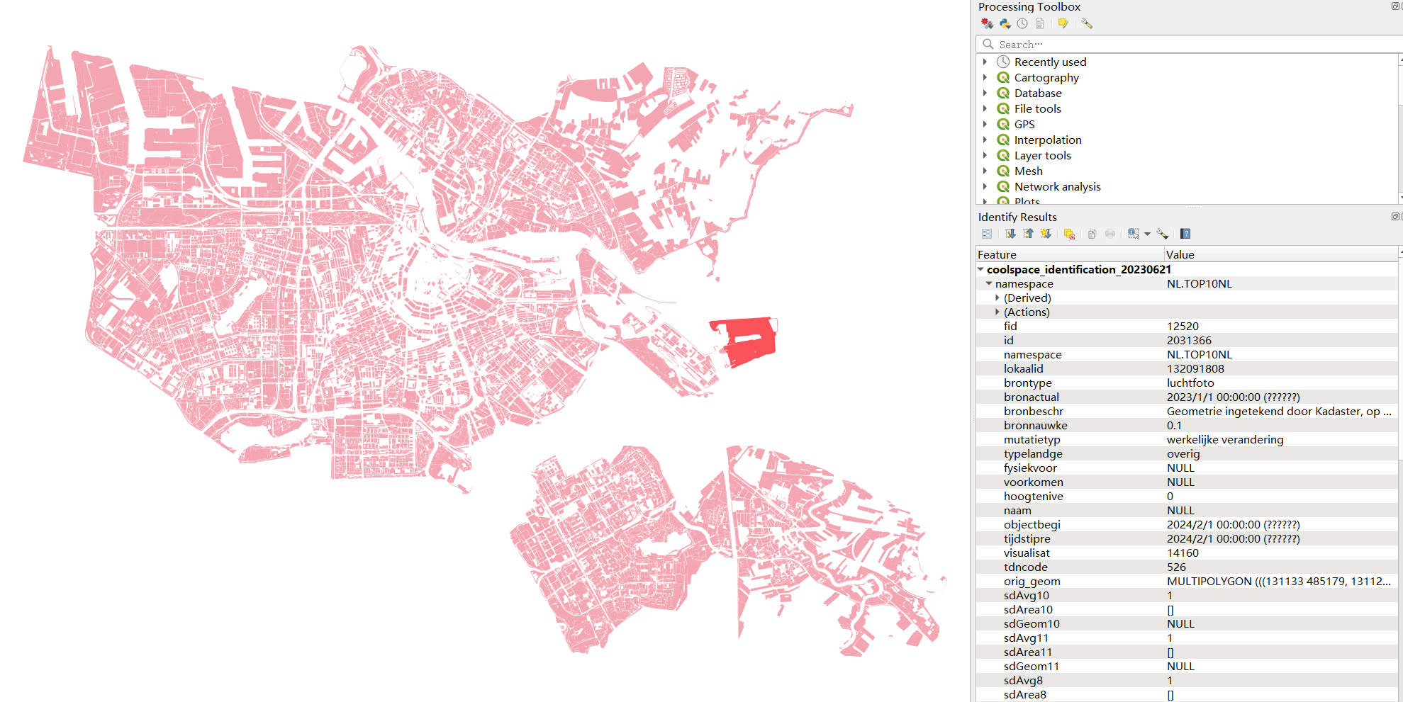
Figure 10: Identification output, geometry type: land use

3. Evaluation

After acquiring the shade geometries from cool spaces candidates, this module evaluate the cool spaces based on the following indicators: shading, usability, capacity, heat risk, and Physiological Equivalent Temperature (PET). The output will be cool spaces polygon with their evaluation attributes for their each shade geometries index. The average of overall scores of shade geometries are calculated in order to make final recommendations , which divided into three categories: Highly Recommended, Recommended, and Not Recommended.

The program will run as:

1. Read the input dataset from main.py of cool space along user parameters from coolspaceConfig.json
2. Call the evaluation function in coolspace_process.py that will be connected to CoolEval.py
3. The following process will be executed:
   • open the data set, read the shade geometries in WKT format and convert it into shape geometries
   • calculate_walkingshed: assigning nearest cool space id for each building -> c_id
   • evaluate_resident: calculating resident for each cool spaces -> resident for number of resident, along with vulnerable group: elder_resi for elders, and kid for children
   • for each shade geometry, iteratively processing:
     • evaluate_capacity: calculate capacity per area cap_area and service capacity cap_status
     • evaluate_sfurniture: count number of benches Benches
     • evaluate_heatrisk: average heat risk heat_rs and classified heat risk heat_rlv from dataset
     • eval_pet: average PET value from raster dataset PET **note: for PET evaluation, since the current PET dataset in this project was made in July 1st, thus it is recommended to use PET only for June or July, since it will not be reliable for the other month. thus, the weight of PET for evaluation can be changed accordingly as user parameter, where user can put the parameter with no more than 0.15 and the default parameter is 0.
4. Aggregate all those evaluation attributes back to cool spaces and average them
5. Make final recommendation for cool spaces with three different shade coverage indicator:
   • final_recom : combining sc and sp as shade indicator
   • final_recom_sc : using sc as shade indicator
   • final_recom_sp: using sp as shade indicator
6. The output will be exported into a geopackage file.

---

OUTPUT

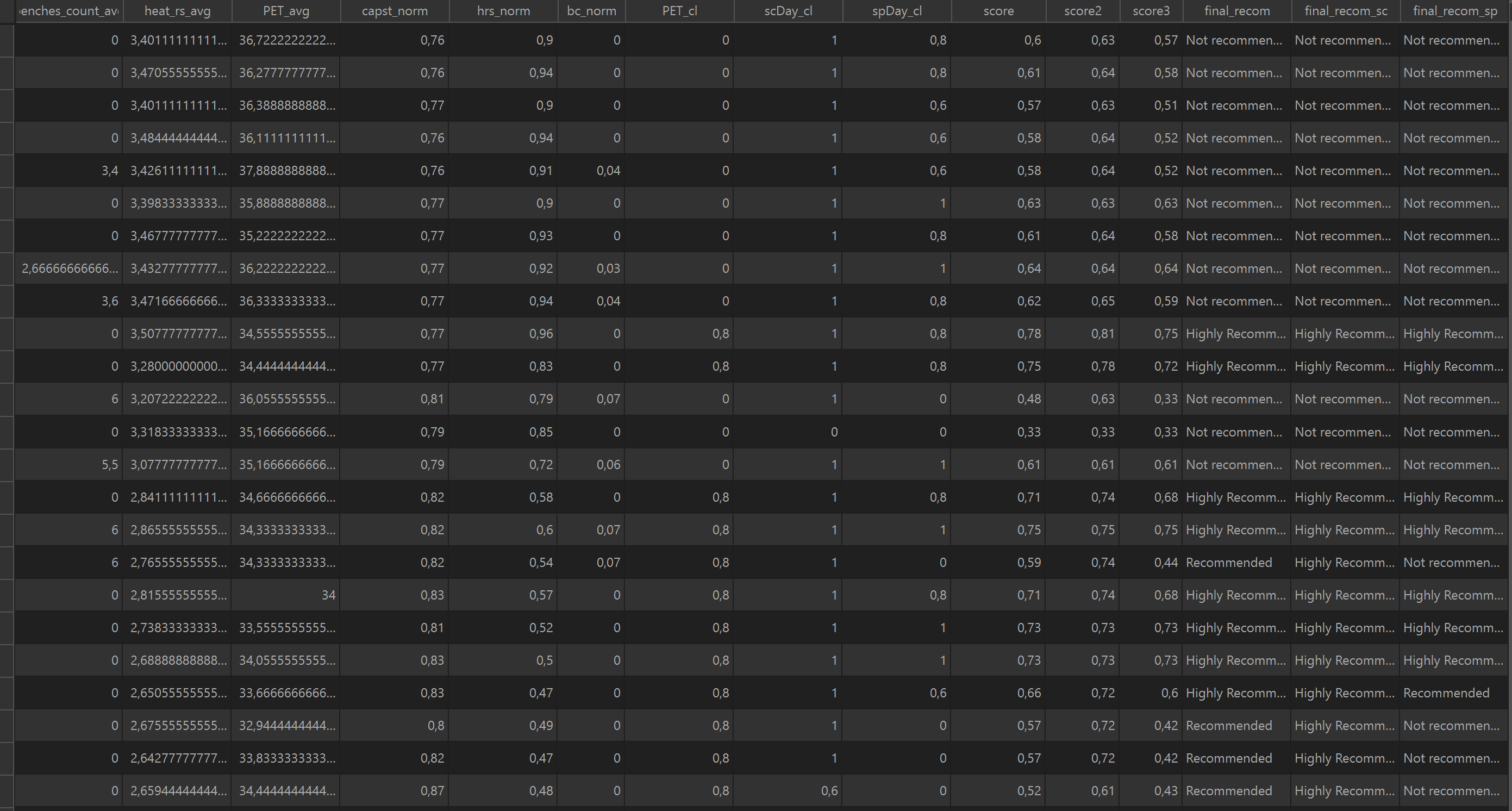
Figure 11: Evaluation output: Attribute table

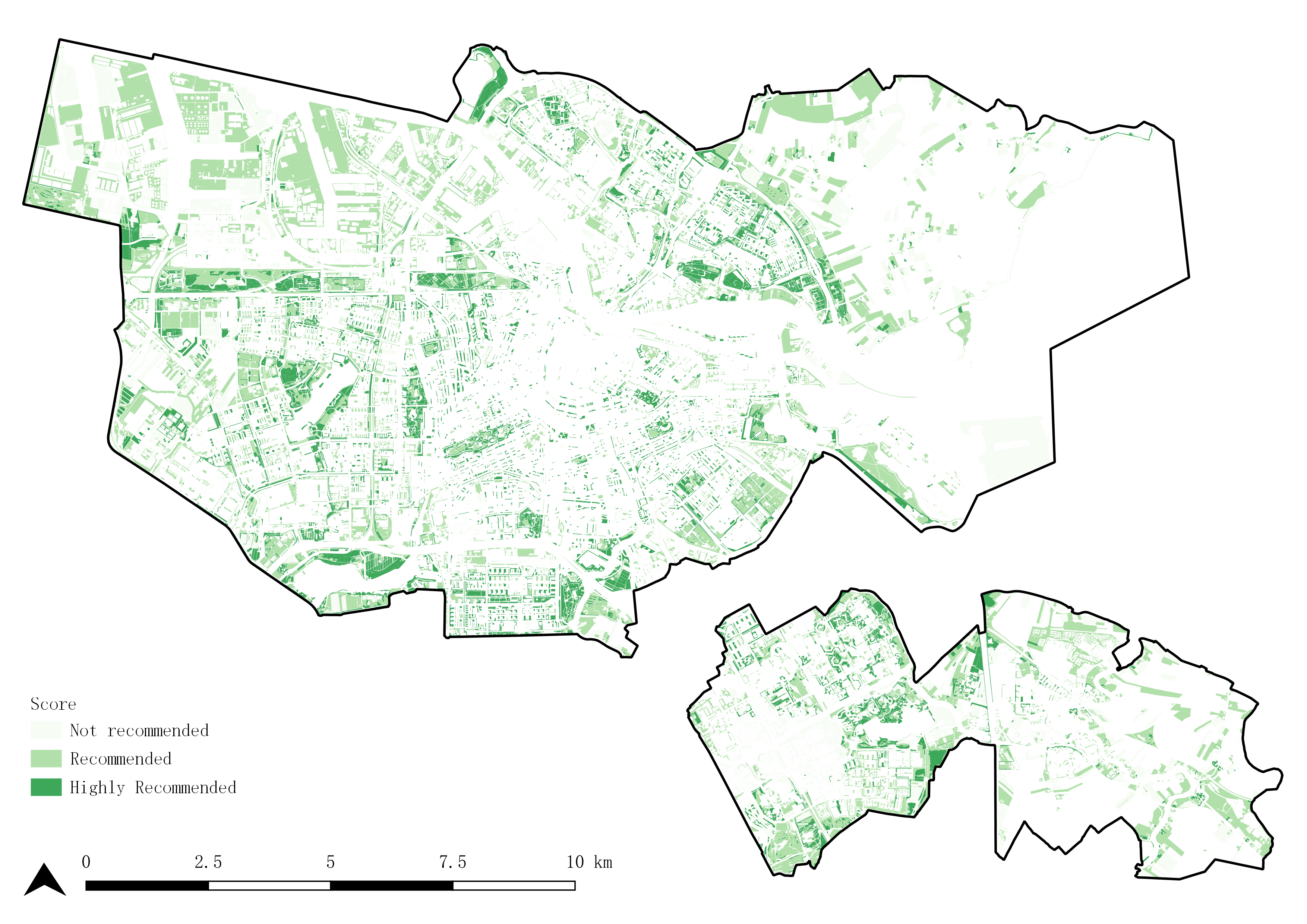
Figure 12: Evaluation output: Recommendation map

This site is open source. Improve this page.